16 Power and Sample Size
The previous chapter covered who should be in your study and how to enroll them. This chapter takes up a different question: how many participants do you need?
The number has to be calibrated, because errors in either direction are costly. Too few participants and your study can’t reliably detect the effect it was designed to find, so the most likely outcome is an inconclusive result. Too many and you’re spending time, money, and participant burden the question doesn’t require. This is the Goldilocks problem of sample size: the target is just right, large enough to answer your research question reliably and small enough to be feasible under real-world constraints.
Sample size is also an ethical decision. Halpern and colleagues argued that underpowered trials are unethical: participants accept the risks and burdens of research while the study is unlikely to produce knowledge that justifies them (Halpern et al., 2002). Oversized studies raise a parallel concern in resource-constrained settings, where every unnecessary participant absorbs funding and staff time that could serve patient care or other research.
What counts as just right depends on what you’re trying to learn. Forty participants is wholly inadequate for a trial designed to detect a reduction in maternal mortality, but may be more than enough for an in-depth qualitative study of women’s experiences of pregnancy. A sample that produces a precise prevalence estimate can be far too small to detect whether an intervention works. The same number can be too many for one question and too few for another, so this chapter organizes sample size around the kind of question you’re asking.
16.1 The Three Buckets of “How Many?”
“How many?” can’t be answered until you’ve answered a prior question: what are you trying to find out? The right approach to sample size follows from the research question, and research questions sort into three buckets, each with its own logic:
Bucket 1: Qualitative Research asks “how many interviews, focus groups, or observations until I’ve captured the depth and diversity of experiences?” The answer comes from the concept of saturation—you keep collecting data until you stop hearing new themes, new perspectives, new dimensions of the phenomenon. Sample size isn’t predetermined; it emerges from the iterative process of data collection and analysis.
Bucket 2: Descriptive Quantitative Research asks “how precisely do I need to estimate this quantity?” If you’re measuring disease prevalence, intervention coverage, or health system characteristics, you’re trying to estimate a number with an acceptable margin of error. Your sample size calculation balances how precise you want your estimate to be against how many people you can actually reach.
Bucket 3: Hypothesis-Testing Research asks “how confident do I want to be that I’ll detect an effect if it exists?” This is the domain of power analysis—you’re calculating how many participants you need to have a reasonable chance (typically 80%) of finding a statistically significant result if your hypothesis is true.
No bucket is better than another; the task is matching the approach to your question. The next three sections take each bucket in turn, using real examples from global health research in low- and middle-income countries.
16.2 Bucket 1: Qualitative Studies—Sampling Until Saturation
If you’re conducting qualitative research—interviews, focus groups, ethnographic observation—you’re not trying to estimate a number or test a hypothesis. You’re trying to understand the complexity, depth, and diversity of a phenomenon. How do community health workers experience their roles? What barriers do women face in accessing maternal healthcare? How do families navigate dementia care without formal support systems? For these questions, the concept of saturation guides sample size determination.
WHAT SATURATION ACTUALLY MEANS
Saturation sounds simple: you’ve reached it when collecting more data yields no new information. But the word covers four distinct ideas, each reached at a different stage of the research and judged by a different standard (Rahimi et al., 2024). Knowing which one you mean keeps “we reached saturation” from becoming an empty claim.
Data saturation
Data saturation is reached when new interviews or observations stop adding information that bears on your research question. Picture interviewing patients who stopped tuberculosis treatment before finishing. The first interviews surface a stream of new reasons: the cost of travelling to the clinic, side effects, feeling better and assuming the cure was done, stigma from neighbors. After fifteen or so, a new patient names only reasons you have already recorded and nothing you haven’t. That is data saturation: the data confirm the picture rather than extend it. Because it is judged during data collection, it is the weakest of the four on its own. The patterns and relationships that matter can still shift once you analyze the transcripts in depth.
Tran and colleagues reached saturation this way in their study of dementia caregivers in Hanoi (Tran et al., 2025). Interviewing 20 caregiver dyads and 8 health professionals across two rounds, they continued “until evidence became redundant with no new information emerging” and identified data saturation after the twentieth interview.
Code or thematic saturation
Qualitative analysis works by coding: researchers attach a short label to each segment of text that captures a recurring idea, then group related codes into broader themes. Code saturation is judged later, during analysis. You’ve reached it when further coding produces no new codes or themes, and no new relationships among them. It is more demanding than data saturation, but it can arrive before you understand how the codes connect, and it usually takes more interviews than researchers expect.
Squire and colleagues (2024) examined five virtual interview studies and found that full code saturation arrived late: across the studies, not until 91% to 100% of the planned interviews were complete. In some, that meant the very last interview. Most of the core codes, though, showed up far earlier, at roughly 15 to 23 interviews—just where teams are tempted to stop. The practical safeguard is a saturation matrix that logs when each new code first appears. If three consecutive interviews add no new codes, the claim stands on firmer ground than if you stopped the first time themes began to repeat.
Meaning saturation
Meaning saturation is about depth rather than breadth. Code saturation tells you the labels have stopped multiplying; meaning saturation asks whether you yet understand what each one means. Suppose you are interviewing community health workers about the barriers they face. After a handful of interviews the same codes keep recurring, “lack of supplies” and “difficult travel,” and you are tempted to stop. But do you yet know why supplies run short, or what “difficult travel” actually involves: seasonal flooding, the cost of transport, or safety on the road? Until your reading of a theme stops shifting, you have repetition, not meaning saturation.
In Ramukumba’s (2020) focus-group study of community health workers in South Africa, “lack of support” surfaced in the first of three focus groups with 46 workers and kept recurring; as a code it was saturated early. But the team reached meaning saturation only once they had unpacked what that lack consisted of: unpredictable remuneration, heavy workloads, and limited recognition from the health system of what these workers actually do. What mattered was not that the phrase repeated but that these dimensions, and how they related, became clear only through sustained analysis across the groups. Stopping at the recurring label would have recorded that workers felt unsupported without ever explaining the shape of that feeling.
Theoretical saturation
Theoretical saturation is the original grounded-theory sense, and the most demanding. You reach it when the theory you’re building is complete: no new data alters its concepts, categories, or the relationships among them, and the theory accounts for the evidence you have (Rahimi et al., 2024). It depends on theoretical sampling: deliberately recruiting the cases most likely to challenge or extend the emerging model. A study building a theory of how families decide when to seek care, for instance, would keep recruiting different kinds of families until the model explained each new case and fresh cases stopped reshaping it.
Negative cases—instances that don’t fit your emerging patterns—are gold in qualitative research. If 11 of 12 CHWs feel undervalued but the 12th feels deeply supported, that outlier helps you refine your themes and identify boundary conditions. Actively seek out and analyze these cases.
THE GOLDILOCKS FRAME FOR QUALITATIVE RESEARCH
So what does “just right” mean for qualitative sample size?
Too small: You miss important perspectives, your thematic development is incomplete, and you can’t distinguish between individual idiosyncrasies and broader patterns. Your findings lack credibility because readers wonder whether different themes would have emerged with more participants.
Too large: You’re collecting redundant data that doesn’t add new understanding, overburdening yourself with unnecessary analysis, and potentially exploiting participants’ time when you’ve already learned what you need to know.
Just right: You’ve achieved saturation across the dimensions that matter for your research question, captured a sufficient diversity of perspectives, and can demonstrate through systematic analysis that additional data collection would be redundant rather than revelatory.
The sample sizes in our examples—46 community health workers in one study, 20 caregiver dyads plus 8 health professionals in another—reflect this principle in action. None of these numbers came from a formula. They emerged from rigorous, iterative analysis showing that saturation had been achieved.
16.3 Bucket 2: Descriptive Inference—Sample Size for Precision
Now let’s shift gears entirely. Qualitative research determines sample size through saturation, but what if you’re trying to estimate a quantity?
Descriptive studies in global health aim to establish the frequency and distribution of health conditions, risk factors, or health system characteristics. What’s the prevalence of tuberculosis in indigenous populations? What proportion of TB contacts develop active disease when screened? How common is exclusive breastfeeding at six months?
For these questions, sample size determination focuses on precision. Specifically, the margin of error or width of confidence intervals around your point estimate.
UNDERSTANDING MARGIN OF ERROR
Suppose you want to estimate the prevalence of active tuberculosis in a particular population. You conduct a survey and find that 3% of your sample has active TB. But here’s the thing: that 3% is an estimate based on your sample. The true population prevalence might be a bit higher or a bit lower.
The confidence interval is the band of prevalence values your data can’t rule out. If a survey puts the estimate at 3% with a 95% confidence interval of 2.6% to 3.4%, values inside that band are consistent with what you observed and values outside it are not. The width of that interval—here 0.8 percentage points—reflects your precision.
The 95% in a confidence interval refers to the long-run behavior of the procedure that produced it, not to this one interval. Chapter 6 works through what that means, and how it differs from a Bayesian credible interval.
A narrower confidence interval means more precision: you can pin down the true value more exactly. But narrower confidence intervals require larger sample sizes. Wider confidence intervals mean less precision but require smaller samples.
Here’s where the Goldilocks problem emerges: In low- and middle-income countries where sample size calculations must be balanced against resource constraints and recruitment feasibility, you need to carefully specify an acceptable margin of error. Too wide a margin produces imprecise estimates that may not be useful for decision-making. Too narrow a margin may make your study completely infeasible.
EXAMPLE: TWO MALARIA SURVEYS IN MOZAMBIQUE
One way to see precision at work is to compare two studies of the same disease that made very different choices about sample size. We’ll discuss two examples that estimated Plasmodium falciparum malaria prevalence in Mozambique:
- a national estimate drew on the 2018 Malaria Indicator Survey, which tested 4,347 young children across the country, and put prevalence at 38.9% (95% CI: 36.9%–40.8%) (Ejigu, 2020);
- a district study in rural Sussundenga tested 358 people from 96 households and put local prevalence at 31.6% (95% CI: 26.6%–36.5%) (Earland et al., 2022).
Look at the two intervals. The national estimate spans 3.9 percentage points; the district estimate spans 9.9, more than twice as wide. The difference is sample size. With roughly twelve times as many people tested, the national survey pins prevalence down far more tightly.
That precision has a price. The national figure took the machinery of a countrywide survey, hundreds of clusters and thousands of tests. The district team could field a study of 358 people with far less, but their estimate is correspondingly coarser. Neither is wrong. They answer questions at different scales, and each accepted the margin of error its purpose and resources allowed.
PROPORTIONS
The Mozambique surveys estimate a proportion: the share of people who test positive for malaria. Both used rapid diagnostic tests, which detect a current infection, so the estimate is a point prevalence: the proportion infected at the time of the survey, not over some earlier period.
For a proportion, the margin of error has a simple form. If you draw a simple random sample of size \(n\) and observe a proportion \(p\), the 95% margin of error is approximately
\[\text{ME} = 1.96 \sqrt{\frac{p(1-p)}{n}}.\]
Two things drive it. The numerator, \(p(1-p)\), is the variability of a yes-or-no answer. It is largest when \(p = 0.5\) and shrinks as prevalence moves toward 0 or 1. The denominator is your sample size. Because \(n\) sits under a square root, precision improves only with the square root of effort: to halve your margin of error you need four times the sample.
Rearranging tells you the sample size a target margin of error requires:
\[n = \frac{1.96^2 \, p(1-p)}{\text{ME}^2}.\]
When you don’t yet know the prevalence, use \(p = 0.5\). It is the worst case, so the resulting sample size is safe for any true value. Figure 16.1 shows what that demand looks like as you ask for more and more precision.
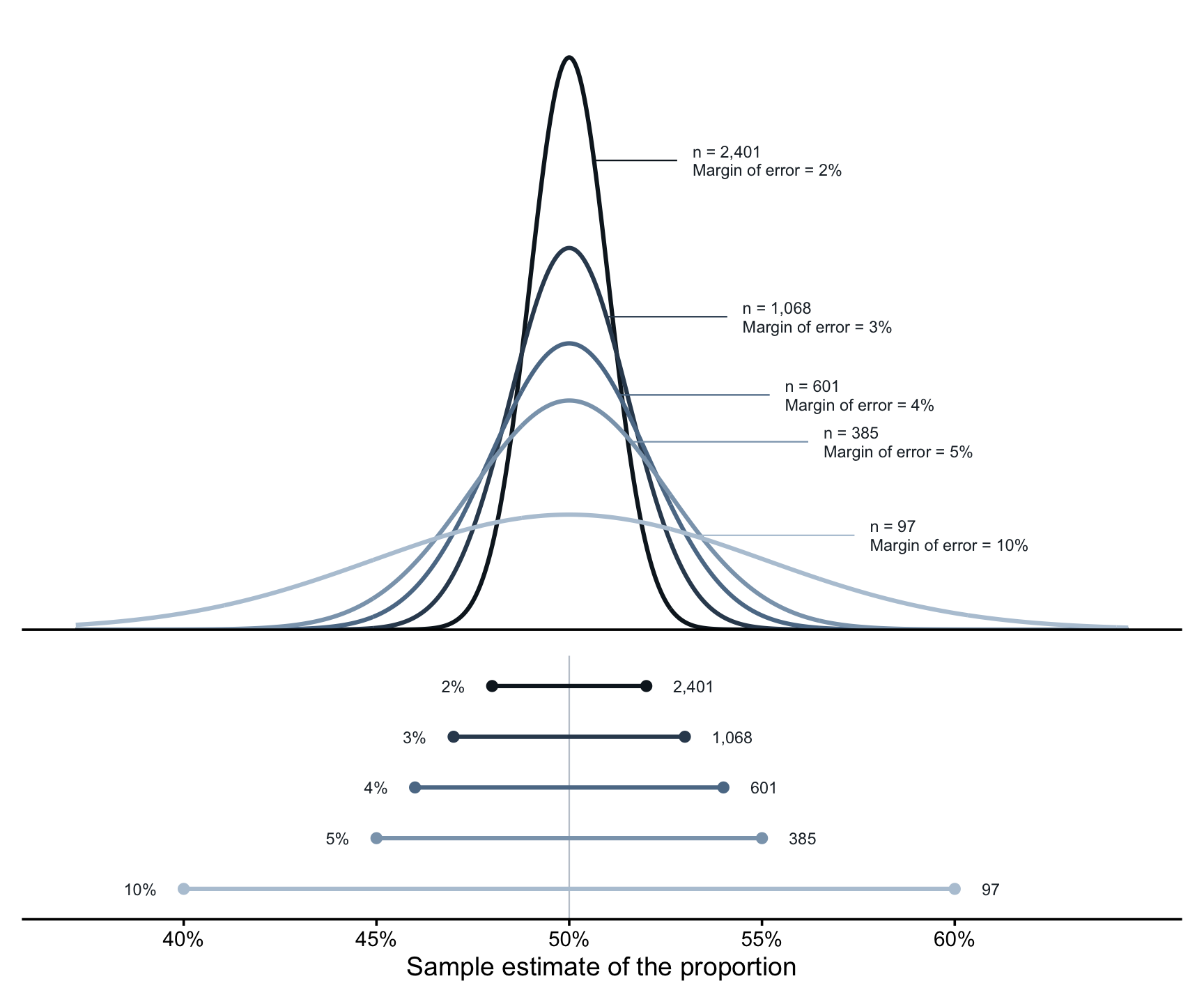
The top panel shows how estimates from repeated samples would scatter around the truth. A small sample gives a wide, flat distribution: with 97 people, a sample could easily land ten points away from the true value. Each increase in sample size pulls that distribution tighter, and the bottom panel translates the same information into the interval each sample size produces.
Notice how unevenly the cost falls. Moving from a 10-point margin to a 5-point margin costs about 290 extra participants. Moving from 5 points to 2 costs about 2,000 more. Malaria’s roughly 39% prevalence makes \(p(1-p)\) a little smaller than the worst case shown here, so the true requirement is somewhat lower, but the shape is the same. This is why a district team of a few hundred can report a usable estimate while a tightly bounded national figure needs a survey of thousands.
MEANS
Sometimes the quantity you want is a mean rather than a proportion: average systolic blood pressure in a community, average out-of-pocket spending on a hospital visit, or average hemoglobin concentration in an anemia screening program. The logic carries over, with one change.
For a mean estimated from a simple random sample, the 95% margin of error is approximately
\[\text{ME} = 1.96 \, \frac{s}{\sqrt{n}},\]
where \(s\) is the standard deviation of the measurement in the population. Rearranged,
\[n = \left( \frac{1.96 \, s}{\text{ME}} \right)^2.\]
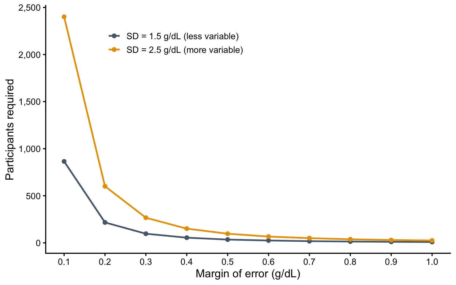
The square-root relationship is unchanged: quadruple the sample to halve the margin of error. What is new is \(s\). For a proportion, variability is fixed once you know \(p\). For a mean, it depends on how spread out the values are, and you have to supply that number before collecting any data. You get it from a previous study in a similar population, from a pilot, or from a conservative guess. Get it badly wrong and your study ends up over- or under-sized for the precision you wanted.
The standard deviation measures how spread out individual values are around their mean. In a homogeneous population, most people sit close to the average and the standard deviation is small. In a variable one, values scatter widely and it is large. It is the standard deviation of the measurements themselves, not the standard error of the estimate. The two are related by \(\text{SE} = s / \sqrt{n}\).
Figure 16.2 makes the point with hemoglobin concentration. The two curves assume a fairly homogeneous population (a standard deviation of 1.5 g/dL) and a more variable one (2.5 g/dL). The more variable population needs a larger sample for the same precision, which is why the standard deviation you assume at the design stage is worth getting right.
THE GOLDILOCKS FRAME FOR DESCRIPTIVE STUDIES
So what’s “just right” for descriptive quantitative research?
Too small: With a small sample size, your confidence intervals are so wide that the estimate provides little useful information. Knowing TB prevalence is “somewhere between 10% and 40%” doesn’t help anyone plan interventions.
Too large: On the flip side, you could recruit nearly 10,000 people to estimate prevalence within 1 percentage point, when a plus/minus of 2 percentage points would have answered your question at a fraction of the cost and effort.
Just right: The just right sample size is the one that answers your question with a tolerable amount of error.
Think about your research in context. Are you providing the first prevalence estimate in a population where none exists? A wider margin of error might be acceptable. Are you detecting small changes over time to evaluate a program? You might need greater precision. Talk to the people who will use your data—public health officials, program managers, clinicians—and ask: “What level of precision would actually be useful to you?” Then design your study accordingly.
16.4 Bucket 3: Hypothesis Testing—The Heart of Power Analysis
Now we arrive at the bucket that causes the most confusion and the most serious errors in research design: hypothesis-testing studies that require power analysis.
If you’re conducting a randomized trial, a cohort study comparing exposed and unexposed groups, or a case-control study investigating risk factors, you’re testing a hypothesis about whether an effect exists. Does an intervention reduce depression? Does exposure to indoor air pollution increase respiratory infections? Do maternal education programs improve child nutrition?
These questions change what “how many?” means. You’re no longer estimating a single quantity to a chosen precision. You’re trying to detect something—a difference between groups, an association—that may or may not be there. The sample size question becomes: how many participants give you a good chance of finding the effect if it really exists? That chance is called power, and before we calculate anything, I want you to have an intuition for what it is.
Several ideas in this bucket—justifying error rates rather than defaulting to convention, the smallest effect size of interest, sensitivity power analysis—come from Daniël Lakens’ open-access chapter on sample size justification (Lakens, 2022). When you’re ready to go deeper than we can here, start there.
A HYPOTHESIS TESTING REFRESHER
To get where we’re going, we need to return to the logic of hypothesis testing from Chapter 6. We assume the null hypothesis of no effect and ask how surprising our data would be if that assumption were true.
For instance, if a prenatal nutrition intervention really had no effect on average newborn birthweight, we’d expect the intervention and control arms to have the same mean birthweight, apart from chance variation. A mean difference of zero.
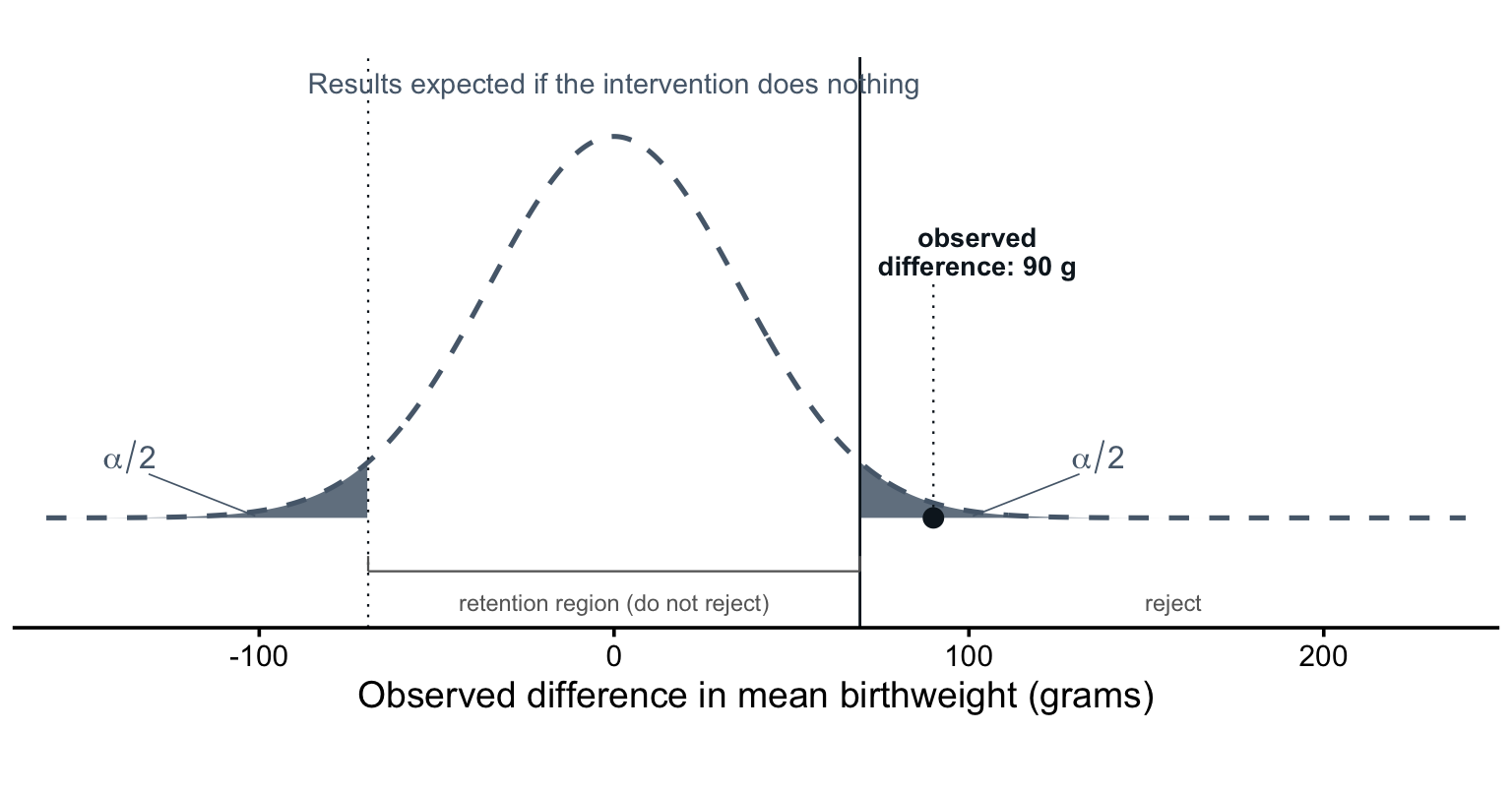
But suppose we observed an average difference of 90 grams between the arms, with a p-value of 0.011. If we had set alpha at 0.05, we’d reject the null hypothesis and conclude that the data provide evidence of an effect. A mean difference of 90 grams—our study result—would be sufficiently surprising under the assumption that the intervention had no effect.
As Chapter 6 emphasized, whether an effect exists is not the only question—or even the most important one. The size of the effect and its clinical or practical significance matter more for decisions. I’m setting that aside here to focus on the testing procedure.
Figure 16.3 draws that reasoning. The dashed curve is the range of results a trial of this size would produce if the intervention truly did nothing: mostly small differences scattered around zero, because two arms drawn from the same population rarely have identical means. Alpha marks off the tails, our threshold for what we’ll consider “surprising.” Anything inside the bracketed retention region is ordinary enough that we don’t reject the null; anything past it is surprising enough that we do. Our 90-gram result sits outside. Therefore, we label it “statistically significant.”
NoteWhat Determines the Shape of The Curve?
The shape of this curve comes from the central limit theorem (Chapter 6). Differences in sample means follow an approximately normal distribution, and its spread depends on just two things: the variability of birthweight and the sample size. With a standard deviation of 500 grams and 400 women per arm, the standard error is \(500 \times \sqrt{2/400} \approx 35\) grams. Enroll more women and the curve narrows.
INTRODUCING POWER
We needed this refresher because the Frequentist hypothesis testing procedure runs entirely on the null hypothesis. The curve in Figure 16.3 describes the plausible results we can expect even if the intervention does not work. The alpha thresholds delineate our automatic decision-making about statistical significance. Inside = not significant. Outside = significant.
Even as someone new to statistical inference, you can see that it’s better to be outside the null distribution retention region if you think an intervention works, or if you believe an association is real.
So how do we design studies where we have the best chance of detecting a result that is outside rather than inside? The answer gets us to the idea of statistical power.
To help me explain power, I created Figure 16.4 that keeps the distribution of plausible study results under the null hypothesis and adds the range of results we might expect if the maternal nutrition intervention really does raise birthweight by 100 grams.
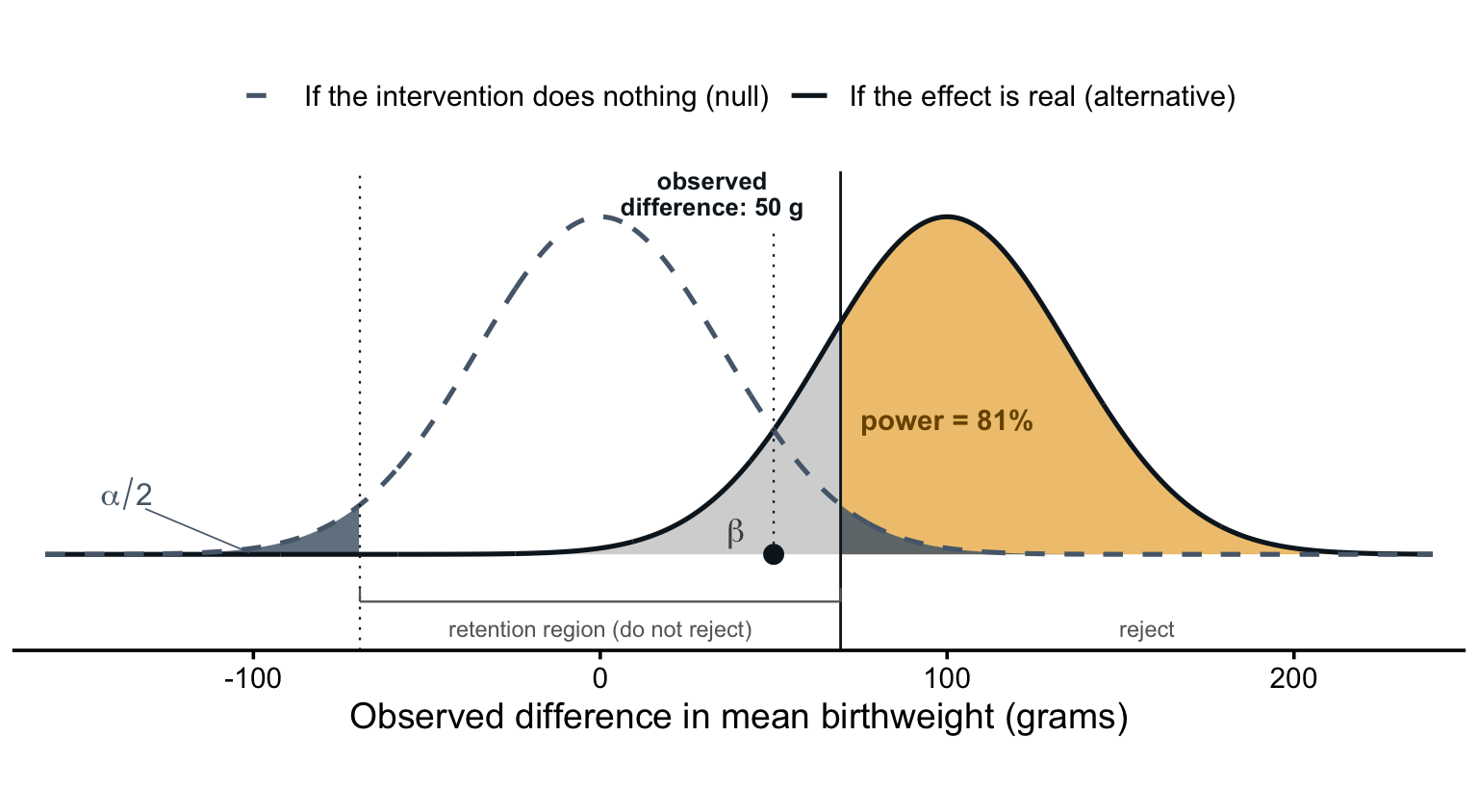
Focus on the hump to the right. Notice how the curve is centered on a difference of 100 grams instead of zero (no effect). But also notice that the two distributions overlap because even in a world where the intervention increases birthweight by 100 grams, sampling variability means that we could see results above or below this mark.
Imagine that our study found a mean difference of 50 grams. An effect of this size falls inside the retention region of the null distribution, so the inferential procedure is clear and automatic: we retain the null. We label the result not statistically significant. Its position on the null distribution tells us that a difference of 50 grams is not all that surprising if the intervention really has no effect.
But look where 50 grams sits on the solid curve.
If the intervention truly raised birthweight by 100 grams, a result of 50 grams would also not be out of the question!
In fact, 50 grams sits exactly midway between the two curves, so this result is just as likely in a world where the intervention truly raises birthweight by 100 grams as in a world where it does nothing.
Hypothesis testing happens on the null hypothesis, so we’d label this particular result not statistically significant. But if the effect is real, that retention is a false negative, otherwise known as a Type II error.
The light gray area in Figure 16.4 shows how often that mistake would happen. I’ve labeled it beta: the share of the real-effect curve that falls inside the retention region, here 19% of the total area under the alternative distribution. Nearly one in five trials of this design would miss a true 100-gram effect. That is to say that nearly 20% of plausible results under the alternative hypothesis also fall inside the null distribution’s retention region. The null wins, and these results get labeled not significant.
The amber area is power: the share of real-effect trials that clear the critical value and correctly reject the null, 81%. The greater the power, the greater the chance you have when designing a study to find an effect if the effect is real.
I know, this conditional probability stuff is tiring. It’s key though because in any single study we never know which side of the truth we’re on. If we knew, we wouldn’t need the study.
When we reject the null, as we did after observing a 90-gram difference in Figure 16.3, we could be making a Type I error (false positive) if the intervention really has no effect.
When we retain it, as we just did after observing a 50-gram difference, we could be making a Type II error (false negative) if the opposite is true and the intervention really does work.
Each world produces a range of plausible results. When these ranges overlap, a single result often can’t tell us which world produced it.
So the question for us designing studies becomes, “How can we design a study so that the distributions overlap as little as possible?” In other words, how do we design high-powered studies?
LEVERS OF POWER
We can’t control which world is true, but we can control the design. Every element of Figure 16.4 comes from a quantity we choose or estimate before enrolling a single participant:
- effect size
- variability
- sample size
- alpha level
- power
Effect Size
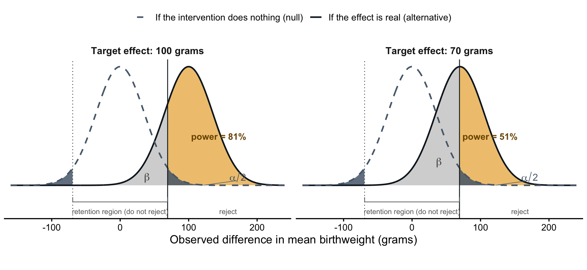
We’ll start with the effect size, which sets the center of the solid curve. It’s the true difference between arms in a world where the intervention works—here, 100 grams. We hypothesize it from past studies, pilot data, or the smallest difference that would matter in practice. The value we choose is our minimum detectable effect size: the smallest true effect the design would reliably detect. Figure 16.5 shows the choice at work. With 400 women per arm and a two-sided alpha of 0.05, the trial has 81% power to detect an effect of 100 grams or greater. If we want to detect a smaller impact, say 70 grams, the same design gives us only 51% power. The curves overlap more, and about half of such studies would miss a real 70-gram effect. Detecting smaller effects takes a different design.
For continuous outcomes you’ll often see effect sizes standardized: the difference in means divided by the standard deviation of the outcome. A 100-gram difference against a 500-gram standard deviation is a standardized effect of 0.2. We’ll stay in grams.
Variability
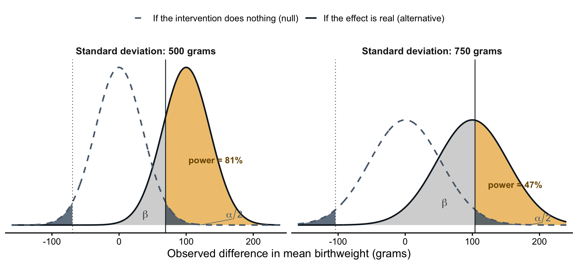
Next is the variability of the outcome, by which we mean how much the outcome differs from person to person before any intervention enters the picture. Birthweight varies a lot. With a standard deviation of 500 grams, one newborn might weigh 2,800 grams and the next 3,700, even when their mothers received identical care. That person-to-person spread is the noise a 100-gram treatment signal has to stand out against, and it’s what gives the curves their width: the more variable the outcome, the wider both distributions and the more the two worlds overlap. Figure 16.6 shows this lever alone. Both panels keep the target effect at 100 grams and the sample at 400 women per arm; only the standard deviation changes. At 500 grams, the value we’ve been assuming, power is 81%. At 750 grams, both curves widen, the two worlds become harder to tell apart, and power falls to 47%.
Variability looks like a fixed fact about the outcome, but analysis choices can shrink it. Adjusting for baseline covariates that predict the outcome—gestational age at enrollment, the mother’s weight, or a baseline measure of the outcome itself—removes the variation those covariates explain. That narrows the curves and buys power without enrolling anyone new. Covariates that don’t predict the outcome buy nothing.
Sample Size
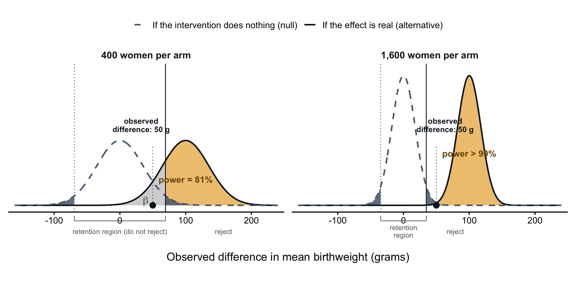
Sample size pushes in the opposite direction. Averages computed from more participants vary less from sample to sample, so enrolling more women narrows both curves. Together, variability and sample size set the standard error—the spread of the distributions. We usually can’t make birthweight less variable, but we can almost always enroll more women, which makes sample size the lever we reach for most often. Figure 16.7 shows it at work. The left panel is the trial we’ve been studying: 400 women per arm, a critical value of 69 grams, and the 50-gram result inside the retention region. The right panel enrolls 1,600 women per arm instead. Both curves grow taller and narrower because results cluster more tightly around each world’s center. The critical value drops to 35 grams, and the same 50-gram result now rejects the null. Power to detect a true 100-gram effect climbs from 81% to more than 99%.
Alpha Level
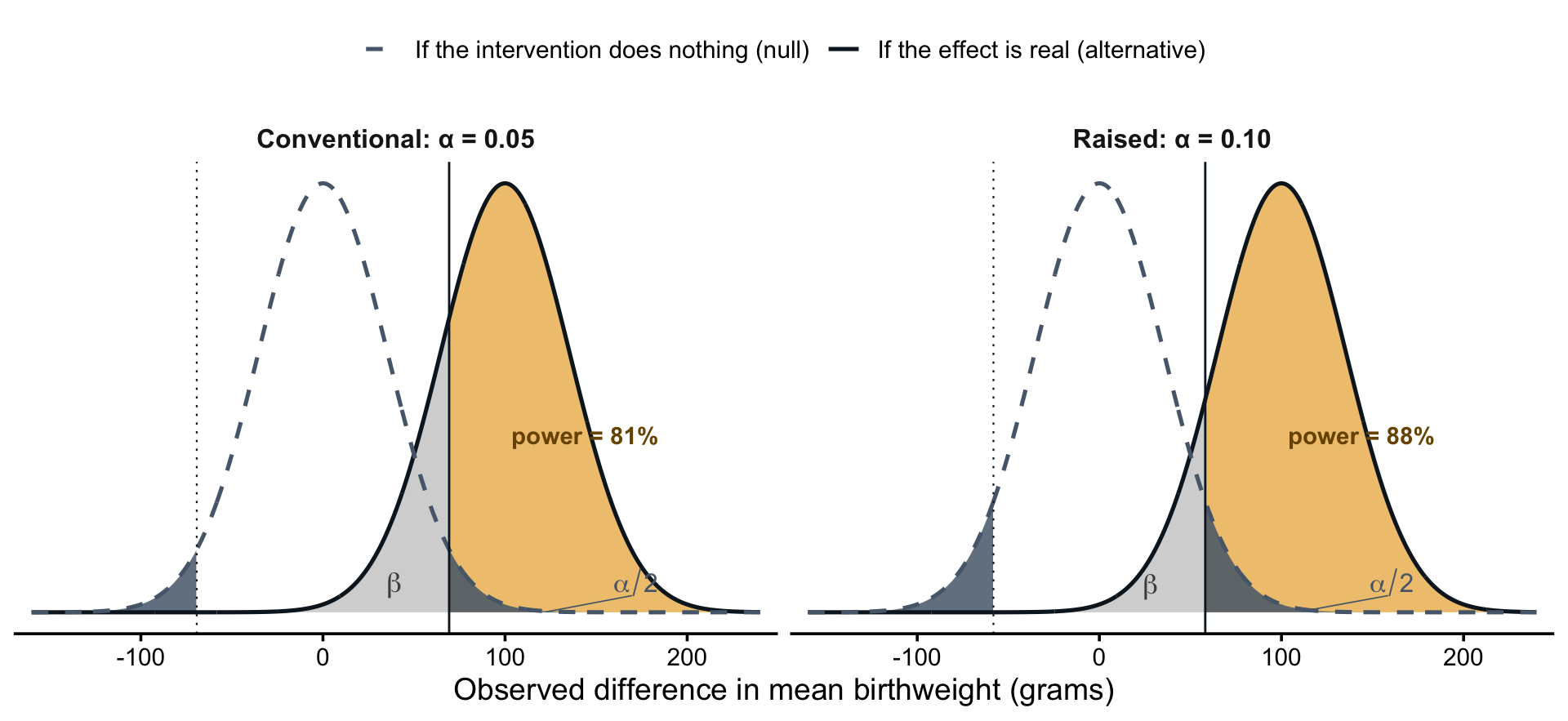
Alpha is the next lever. It sets the critical values: with a two-sided alpha of 0.05, they sit at ±69 grams. There’s nothing special about 0.05. It’s a convention, and researchers set it. If a false negative would be the costlier error—say, when screening candidate interventions to decide which deserve a definitive trial—an alpha of 0.10 can be defensible. Figure 16.8 shows the consequences. Holding everything else fixed, raising alpha from 0.05 to 0.10 moves the critical value inward from 69 grams to 58, and power rises from 81% to 88%. But nothing about the study got more informative. You bought that power by doubling the false-positive risk you’re willing to accept. That’s why the justification for changing alpha has to come from weighing the two errors, never from working backward to the sample size you can afford. And expect reviewers to question anything other than 0.05 regardless.
Power
Once the effect size, variability, sample size, and alpha are fixed, the picture is fully drawn and power falls out of it: the share of the solid curve that clears the critical value, 81% here. But power becomes an input when you flip the question around. Set a target—convention says at least 80%—and solve for the minimum sample size that achieves it. That flipped question is the power analysis: given the effect we care about, the variability we expect, and the alpha we’ll test at, how large must the sample be for a real effect to have a strong chance of being detected?
The 80% convention is a default, not a law. Jacob Cohen, who proposed it, judged a false positive to be four times as serious as a false negative, and he hoped researchers would override the default whenever they could justify a better value (Cohen, 1988).
We can also solve for the minimum detectable effect. Fix the sample size at whatever you can enroll, keep alpha at 0.05 and the power target at 80%, and solve for the smallest effect the design can reliably detect. With 400 women per arm, the answer is 99 grams, which is why the 100-gram design we’ve been drawing has power just above 80%. If the effects that matter in practice are smaller than the answer, you’ve learned something important before enrolling a single participant.
THE LAMP IN THE BASEMENT
If you’re feeling good about power, you might skip to the next section. If it’s still a bit fuzzy, consider this analogy.
Imagine that I ask my kid to find a lamp in the basement. I’m pretty sure it’s down there. He goes down, pokes around, and comes back: “It’s not there.”
Has he shown that the basement contains no lamp? No. He failed to find it, which is a different claim. His report is the household version of p > 0.05: an absence of evidence, not evidence of absence.
I didn’t invent this analogy, but I’ve lost track of where I first came across it.
Now think about what determines whether he finds it.
The size of the lamp. A floor lamp is hard to miss. A small reading light can hide behind a single box. That’s the effect size: large effects announce themselves in the data, and small effects are easy to overlook.
How long he looks. A thirty-second glance from the bottom of the stairs is one thing. Twenty minutes checking every shelf is another. That’s the sample size. More looking means more chances to find what’s there.
How messy the basement is. In a tidy basement, even a small lamp stands out. In a basement crammed with boxes and bikes, a large lamp can sit unnoticed. That’s the variance in your outcome. It also echoes the margin note on the variability lever: if you can account for some of that variation by clearing away clutter that has nothing to do with the lamp, you gain power without enrolling a single extra participant.
Power is the probability that my kid comes back holding the lamp, given that the lamp really is down there. In study terms, it’s the probability of rejecting the null when the effect truly exists. Just like the p-value is conditional on the null hypothesis being true, power is a conditional probability of finding an effect if there is one to find.
EXAMPLE: POWERING THE HEALTHY ACTIVITY PROGRAM TRIAL
For a real power calculation, let’s return to the Healthy Activity Program (HAP), the lay-counsellor treatment for depression in Goa, India, that anchored Chapter 6. The trial randomized individual adults with moderate to severe depression to HAP plus enhanced usual care or enhanced usual care alone. A primary outcome was depression severity on the Beck Depression Inventory (BDI-II) at three months.
Every lever appears in the team’s design. The hardest one came first: the effect size. Meta-analyses of low-intensity psychological interventions for depression had found a summary effect of 0.42 standard deviations, while behavioural interventions overall pooled to 0.7 (Patel et al., 2014). The team designed around the smaller number. That choice cost them participants, but it protected the study: if HAP performed more like the low-intensity treatments, they would still have the power to detect it.
One detail I’m setting aside: HAP participants shared counsellors and clinics, so the team also inflated their target slightly—by a factor of 1.28—to account for the resulting similarity among patients at the same site (Patel et al., 2017). What that adjustment means comes later in this chapter, in the section on cluster randomized trials.
With the effect size fixed at 0.42, the rest followed. They kept alpha at the conventional 0.05, set power at 90% for depression severity (and 92% for the binary remission outcome), and assumed 15% of participants would be lost to follow-up, inflating the target to compensate. The arithmetic pointed to 500 participants, 250 per arm (Patel et al., 2017). They enrolled 495.
The design paid off. The trial found an adjusted mean difference of -7.57 points on the BDI-II, a standardized effect of 0.48—slightly larger than the 0.42 the study was powered to detect. The hypothesized effect was realistic, the sample was large enough to find it, and the trial delivered a clear answer.
Notice what the 0.42 was: an expectation, borrowed from meta-analyses of similar treatments. There’s a second number worth asking about, and it makes for an even stronger justification: the smallest effect size of interest—the smallest effect that would still matter for patients or for the health system. The two numbers answer different questions. Powering for the expected effect tells you whether you can detect the effect if your expectation is right. Powering for the smallest effect that matters does something better: it makes even a null result informative, because any effect the study was likely to miss is smaller than the ones anyone cares about. Arriving at that number takes deliberation with the people who would act on the result. How many BDI-II points must a treatment move, or what remission rate must it reach, before scaling up lay counsellors is worth the cost? That’s hard, and expectations from prior studies are often the practical fallback. But when you can specify the smallest effect of interest, power for it.
Don’t confuse this with the minimum detectable effect size from earlier. The minimum detectable effect size describes the design: the smallest effect your study can reliably find. The smallest effect size of interest describes the decision: the smallest effect anyone would act on. In a well-justified design, the first is no larger than the second.
POWER CALCULATIONS
You rarely need to do this arithmetic by hand. For basic designs—two arms, one primary outcome, individual randomization—free tools handle the standard calculations (Table 16.1).
| Tool | Where it runs | Best for |
|---|---|---|
power.t.test(), power.prop.test() |
Base R | Two-group comparisons of means or proportions; no packages needed |
pwr package |
R | The same territory plus correlations, chi-square, and ANOVA, specified in standardized effect sizes |
| G*Power | Free desktop app | A long menu of tests behind a point-and-click interface; no coding required |
| OpenEpi | Browser | Quick epidemiological calculations, including case-control and cohort designs |
power command |
Stata | Coverage comparable to G*Power for Stata users |
The base R functions cover everything we’ve done so far. Here is the trial we’ve been drawing:
power.t.test(n = 400, delta = 100, sd = 500)
     Two-sample t test power calculation

              n = 400
          delta = 100
             sd = 500
      sig.level = 0.05
          power = 0.8064964
    alternative = two.sided

NOTE: n is number in *each* group
There’s the 81% power we read off the curves. Swap the arguments and the same function answers the other two questions. Specify power = 0.80 and leave out n, and it solves for sample size:
power.t.test(delta = 100, sd = 500, power = 0.80)
     Two-sample t test power calculation

              n = 393.4067
          delta = 100
             sd = 500
      sig.level = 0.05
          power = 0.8
    alternative = two.sided

NOTE: n is number in *each* group
Round up: 394 women per arm. Specify n and power and leave out delta, and it returns the minimum detectable effect—the 99 grams from the previous section.
One more step before a calculated sample size becomes a recruitment target: account for attrition. Power calculations count the participants who provide outcome data, not the ones you enroll. If you expect to lose 15% of participants before the outcome is measured, divide by what remains: 394 / 0.85 = 464 women per arm. Base the expected loss on similar studies in your setting, and build it into the recruitment plan from the start rather than discovering the shortfall at analysis. And remember that attrition can do worse than shrink your sample. If the participants who leave differ from those who stay—especially if they differ across arms—the problem becomes bias, not just power.
Whichever tool you use, check the defaults before trusting the answer: whether alpha is one- or two-sided, whether n means per group or total, and whether the tool expects a raw difference or a standardized effect size. The pwr package, for example, works in Cohen’s standardized units—the d = 0.42 that the HAP team borrowed from meta-analyses plugs in directly.
SIMULATION-BASED POWER ANALYSIS
What happens when your study design gets complicated enough that those simple tools don’t work anymore? Welcome to the world of simulation-based power analysis!
When do you need simulation? Common scenarios include multilevel or hierarchical designs with multiple sources of variation (patients nested in clinics nested in districts), non-normal outcome distributions that violate standard assumptions (count data, highly skewed outcomes), multiple correlated outcomes where you’re testing several related hypotheses, complex intervention effects that vary across subgroups or time points, and missing data patterns that you expect will affect your analysis.
Let me show you the basic logic with a realistic example.
The Basic Logic of Simulation-Based Power
Imagine you’re planning a stepped-wedge cluster randomized trial to evaluate a maternal health intervention across 12 rural health facilities in Uganda. Health facilities will sequentially transition from control to intervention over 18 months, with measurements every 3 months. Your primary outcome is the proportion of women attending at least 4 antenatal care visits.
This design is too complex for standard calculators because it’s a cluster design (facilities, not individuals), it’s stepped-wedge rather than parallel groups, you have repeated measurements over time, the outcome is binary rather than continuous, and you expect correlation within facilities and within time periods.
Simulation lets you answer: “If I enroll X women per facility and randomize Y facilities with this specific design, what’s my probability of detecting a meaningful difference, if one exists?”
Here’s the conceptual approach demonstrated in R:
Step 1: Define your design parameters
# Study design
n_clusters <- 12           # Number of health facilities
n_per_cluster <- 40        # Women enrolled per facility per period
n_steps <- 6               # Crossover steps; baseline + 6 steps = 7 periods
baseline_rate <- 0.45      # Proportion with 4+ ANC visits at baseline
icc <- 0.08                # Intracluster correlation coefficient
n_sims <- 1000             # Number of simulated trials to run

# Target effect: raise ANC attendance from 45% to 60%, expressed on
# the log-odds scale the model works on (a log odds ratio of 0.61)
effect_lor <- qlogis(0.60) - qlogis(0.45)
Step 2: Simulate the data-generating process
To simulate is to generate a fake dataset by drawing random numbers from the model you just specified. Each simulated dataset is one plausible version of your trial—one way the study could turn out if the assumptions in Step 1 are true. For each simulation iteration (typically 1,000 or more):
# Randomly assign each facility a crossover step (2 facilities per step)
cluster_step <- sample(rep(2:(n_steps + 1), each = 2))

# Generate baseline cluster effects
cluster_effects <- rnorm(n_clusters, mean = 0, sd = sqrt(icc))

# Generate time period effects
time_effects <- rnorm(n_steps + 1, mean = 0, sd = 0.05)

# For each cluster and time period, generate outcomes
for (cluster in 1:n_clusters) {
  for (period in 1:(n_steps + 1)) {
    # Determine if cluster has intervention at this time
    intervention_status <- ifelse(period >= cluster_step[cluster], 1, 0)

    # Calculate probability of outcome
    log_odds <- qlogis(baseline_rate) +
                cluster_effects[cluster] +
                time_effects[period] +
                (effect_lor * intervention_status)

    prob <- plogis(log_odds)

    # Generate binary outcomes for n_per_cluster women
    outcomes <- rbinom(n_per_cluster, 1, prob)
  }
}
Step 3: Analyze each simulated dataset
Use the same statistical approach you’ll use in your real study:
# Fit mixed-effects logistic regression
model <- glmer(outcome ~ intervention_status + factor(period) +
               (1 | cluster),
               family = binomial,
               data = simulated_data)

# Extract p-value for intervention effect
p_value <- summary(model)$coefficients["intervention_status", "Pr(>|z|)"]
Step 4: Calculate power
Steps 2 and 3 produce one simulated trial and one p-value. Wrap them in a loop that runs n_sims times, collect the p-values, and count how many fall below your alpha level:
# Run Steps 2-3 n_sims times, keeping the p-value from each trial
p_values <- replicate(n_sims, {
  # ...Step 2: simulate one dataset
  # ...Step 3: fit the model
  p_value
})

# Power = proportion of simulations with p < 0.05
power <- mean(p_values < 0.05)
If power is too low (< 80%), increase your sample size parameters and repeat. If power is very high (> 90%), you might be able to reduce sample size.
Running this loop on the design exactly as specified—12 facilities, 40 women per facility per period—returns power of essentially 100%. A 15-percentage-point improvement is very hard to miss with 3,360 observations, so this design sits in the “power above 90%” branch: we could enroll fewer women. Simulation makes that follow-up question easy to answer. Shrink the enrollment parameter, re-run the loop, and count again.
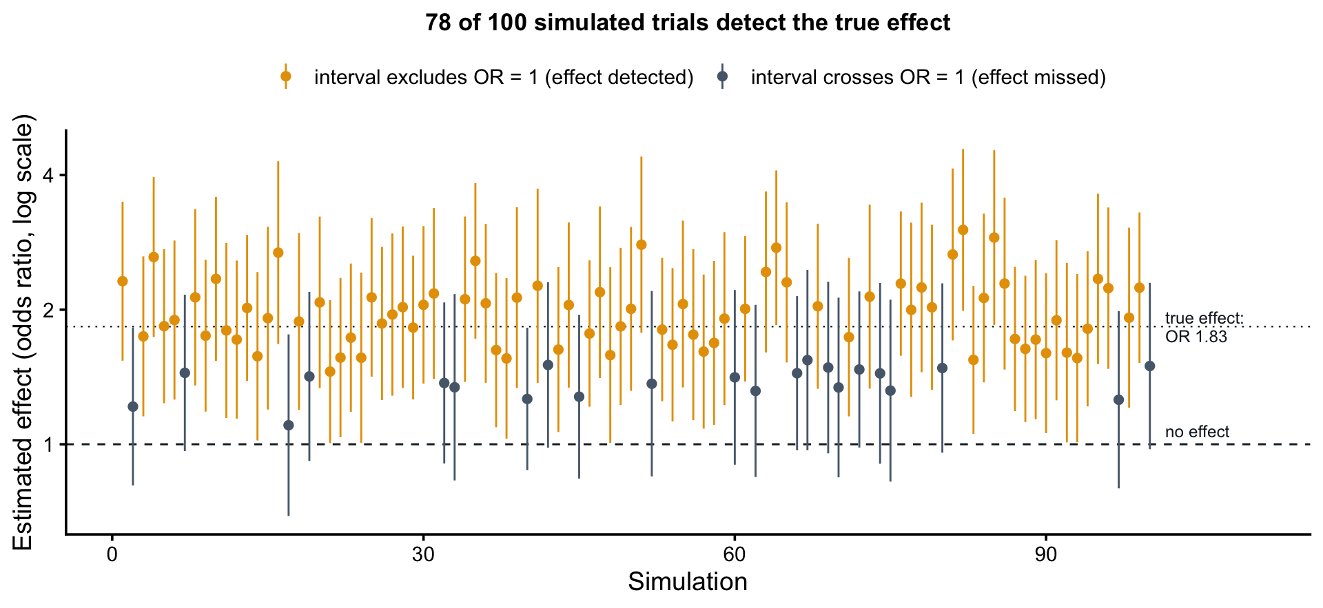
Figure 16.9 shows what this counting looks like with enrollment cut to 10 women per facility per period. Each vertical line is one simulated trial’s estimated intervention effect, an odds ratio from the mixed-effects model in Step 3, with its 95% confidence interval. The estimates bounce around the true effect—that’s sampling variability again—and 78 of the 100 intervals exclude an odds ratio of 1. That count is the simulation’s estimate of power: 78%, just short of the usual 80% target. Enrolling 12 women per facility per period brings power to about 84%, so the team could cut planned enrollment by more than two thirds and still meet the target. More iterations make the estimates more precise; the logic doesn’t change.
What This Reveals That Calculators Can’t
The beauty of simulation is that it handles the messy reality of your specific study design. For this stepped-wedge example, simulation accounts for time trends (what if outcomes are improving regardless of intervention?), variable cluster sizes (what if some facilities enroll 30 women while others enroll 50?), period effects like seasonality in ANC attendance, and the ability to simultaneously assess power for secondary outcomes like skilled birth attendance.
You can also explore “what if” scenarios that standard calculators can’t touch. What if the ICC is actually 0.12 instead of 0.08? What if 20% of participants drop out by the final time point? What if the intervention effect increases over time as facilities gain experience? Simulation answers all of these and lets you game out best and worst case scenarios to inform planning.
SPECIAL TOPIC: CLUSTER RANDOMIZED TRIALS AND THE ICC PROBLEM
We can’t cover power analysis for every design, but one design worth highlighting is the cluster randomized trial.
In a standard randomized trial, you randomize individual participants. In a cluster trial, you randomize at a higher level: villages, health facilities, schools, or geographic areas.
Cluster designs offer major advantages in LMICs. They align with natural service delivery structures and facilitate implementation through existing governance. They reduce contamination between study conditions. And they avoid the ethical concerns that arise when you withhold or delay interventions from some individuals within the same community.
But cluster trials create a methodological challenge: observations within clusters are not independent. People in the same village, treated at the same health facility, or attending the same school tend to be more similar to each other than to people in other clusters. This positive correlation—quantified by the intracluster correlation coefficient (ICC)—violates the independence assumption of standard statistical tests.
Two extreme cases will help to clarify the bounds of the ICC. Suppose you recruit 30 villages of 100 people each, for a total of 3,000 participants. If each village were made up of perfect clones—everyone identical on the outcome, an ICC of 1—then every villager after the first would tell you nothing new. Each village would contribute one independent piece of information. Instead of a sample of 3,000, you’d effectively have a sample of 30. At the other extreme, if the people in a village shared nothing in common—an ICC of 0—the clustering would be irrelevant, and you’d have the power of an individually randomized trial of 3,000.
Understanding the Design Effect
The higher the ICC, the greater the design effect and the greater the sample size needed for the same power.
Design Effect = 1 + (n - 1) \(\times\) ICC
where n is the average cluster size. Divide your actual sample size by the design effect to get your effective sample size. With 100 people per village and an ICC of 0.03, the design effect is 1 + 99 \(\times\) 0.03 = 3.97. Your 3,000 participants provide the information of about 750 independently sampled individuals. Put the other way: this cluster trial needs roughly 4 times the sample size of an individually randomized trial to reach the same power.
Cluster size n multiplies the ICC in the design effect, but the number of clusters appears nowhere in it. Adding people to existing clusters inflates the design effect; adding clusters doesn’t. With 6,000 participants and an ICC of 0.03, 30 villages of 200 give an effective sample of about 860, while 60 villages of 100 give about 1,510. When you can choose, add clusters, not cluster size.
This sample size inflation can be a brutal wake-up call when you’re trying to design feasible research in resource-limited settings.
How Big Are ICCs Really?
You can’t compute a design effect without an ICC, but you won’t observe your trial’s ICC until the data are in. So where does the number come from? Start with the literature. Many published cluster trials report the ICCs they observed, and methodologists have compiled these values across hundreds of trials. Trials with a similar outcome, population, and cluster type give you a plausible starting range.
But nothing beats pilot data. If you can measure your outcome in even a handful of clusters, you can calculate the ICC directly for your population, your clusters, and your instrument. Pilot estimates based on few clusters are noisy, so don’t bet the design on a single value: run the power calculation across a range of ICCs and see how sensitive your sample size is. And when your trial ends, report the ICC you observed. The next team designing a similar study will start from better information than you did.
THE GOLDILOCKS FRAME FOR HYPOTHESIS-TESTING STUDIES
What’s “just right” for hypothesis testing studies?
Too small (underpowered): You have essentially no chance of detecting anything but enormous effects. Your study will almost certainly be inconclusive, wasting everyone’s time and resources. This is both a scientific failure and an ethical problem.
Too large (overpowered): You’ll detect statistically significant differences that have no practical meaning, like finding that an intervention reduces depression scores by 0.1 points on a 27-point scale. You’ve also demanded far more participants than necessary, potentially making your study infeasible or ethically questionable.
Just right (adequately powered): You have approximately 80% probability of detecting effects of the size that would actually matter for practice or policy. Your sample size is large enough to answer your question reliably, but not so large that you’re wasting resources or participant burden.
The key is to engage that effect size question. Don’t just power your study to detect whatever effect size makes your desired sample achievable (“we can recruit 100 people, so let’s see what effect size that detects!”). Instead, think carefully: What magnitude of effect would actually be meaningful? What have similar studies found? What do theory and prior evidence suggest is plausible?
Then design accordingly, even if that makes your study more challenging. If you are limited to a fixed sample size, solve for power and ask what you can learn from your study, and whether it’s worth doing.
NotePower calculations are used when designing studies
Post-hoc power analysis—computing power from the effect size you just observed—is mathematically circular and provides no new information. Post-hoc power is a restatement of the p-value: a result at exactly p = 0.05 always yields post-hoc power near 50%, and a non-significant result always “reveals” low power. If a reviewer requests it, offer a sensitivity power analysis instead: report the smallest effect your sample could detect, then discuss whether your null result more plausibly reflects a true absence or a miss.
16.5 Closing Reflection
This chapter opened with a claim: the same sample size can be too many for one question and too few for another. Now you can see why. For an in-depth qualitative study of women’s experiences of pregnancy, forty interviews may be more than saturation requires—the last ten confirming themes the first thirty established. For a survey estimating prevalence, forty participants produce a margin of error too wide to guide any decision. And for a trial designed to detect a reduction in maternal mortality, forty is not even in the right order of magnitude: a rare outcome and a modest realistic effect push the requirement into the thousands, and if the intervention is delivered community by community, the design effect inflates it further.
Sometimes your sample size planning delivers bad news: the study you can afford can’t detect the answers that matter. The temptation is to work backward—to adjust assumptions until the calculation justifies the sample you already had. The result is a study that looks powered on paper and remains underpowered in fact. Run the honest calculation instead. Fix the sample size at what you can enroll, solve for the minimum detectable effect, and decide whether that study is worth doing. Sometimes it is, with its limits reported plainly. Sometimes the answer is a different design, a longer timeline, more partners—or a different question, like a qualitative study to understand the problem before a trial tries to solve it. Just don’t plow ahead hoping the math changes because it won’t.
So when you plan your next study, remember Goldilocks. Not too big. Not too small. Calibrated to your question, your context, and your resources.
Cohen, J. (1988). Statistical power analysis for the behavioral sciences (2nd ed.). Lawrence Erlbaum Associates.
Earland, D. E. et al. (2022). Plasmodium falciparum community prevalence and health-seeking behaviours in rural sussundenga district, mozambique. Malaria Journal, 21, 305.
Ejigu, B. A. (2020). Geostatistical analysis and mapping of malaria risk in children of mozambique. PLOS ONE, 15(11), e0241680.
Halpern, S. D. et al. (2002). The continuing unethical conduct of underpowered clinical trials. JAMA, 288(3), 358–362.
Kurz, A. S. (2019). Bayesian power analysis: Part I. Prepare to reject H0 with simulation. Blog post.
Lakens, D. (2017). Equivalence Tests: A Practical Primer for t Tests, Correlations, and Meta-Analyses. Social Psychological and Personality Science, 8(4), 355–362.
Lakens, D. (2022). Improving your statistical inferences.
Patel, V. et al. (2014). The effectiveness and cost-effectiveness of lay counsellor-delivered psychological treatments for harmful and dependent drinking and moderate to severe depression in primary care in India: PREMIUM study protocol for randomized controlled trials. Trials, 15, 101.
Patel, V. et al. (2017). The healthy activity program (HAP), a lay counsellor-delivered brief psychological treatment for severe depression, in primary care in india: A randomised controlled trial. The Lancet.
Rahimi, S. et al. (2024). Saturation in qualitative research: An evolutionary concept analysis. International Journal of Nursing Studies Advances.
Ramukumba, M. M. (2020). Exploration of community health workers’ views about in their role and support in primary health care in northern cape, south africa. Journal of Community Health.
Squire, C. M. et al. (2024). Determining an appropriate sample size for qualitative interviews to achieve true and near code saturation: Secondary analysis of data. Journal of Medical Internet Research.
Tran, T. A. et al. (2025). The experience and needs of informal caregivers of people with dementia in rural vietnam: A qualitative study. Annals of Medicine.